
No-hitters are baseball’s holy grail—but do they come with a cost? Hello, class. I’m Professor Saber, and today we’re embarking on a statistical adventure! Our classroom is the ballpark, our blackboard is the box score, and our subject is one of the most tantalizing questions in baseball: what happens to a pitcher after they throw a no-hitter?
Now, before we begin, I know what many of you are already thinking: “But Professor, I’m not good at math!”
But as I always tell my students — it isn’t that you aren’t good at math; it’s that you haven’t been taught math in the way that you learn. So sharpen your pencils, sit back, and get ready to see numbers not as walls of confusion, but as windows into truth. Because today, we won’t just run an analysis together—you’ll learn how to read the results yourself.

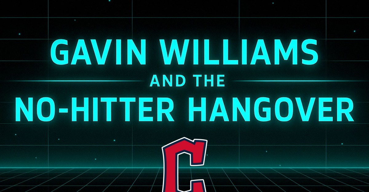
The no-hitter hangover isn’t mere theory, class—we’ve just witnessed the perfect case study in Cleveland. Gavin Williams came within two outs of making history before surrendering a late home run. A Herculean effort, throwing 126 pitches. But was there a price? In his very next start, he didn’t make it past the third inning, giving up four runs, and the Guardians lost the game.
Coincidence—or the inevitable cost of chasing perfection? That’s the quandary we aim to solve today.
And so, my fellow statisticians, we will set out to test the hypothesis: Does flirting with greatness take a toll? Does the arm suffer under the weight of history? Is there such a thing as a No-Hitter Hangover?

Let’s begin with our dataset. We’ll examine every pitcher who threw a no-hitter (including perfect games) in the regular season from 2010–2024. For each pitcher we’ll compare their season averages to their performance in their start immediately following the no-hitter. To do this, we will focus on six key metrics: Innings Pitched (IP), Hits (H), Runs (R), Earned Runs (ER), Strikeouts (K), and Walks (BB).
From 2010 to 2024, there were 50 no-hitters (excluding postseason and combined efforts). However, three of these came in a pitcher’s final start of the season. That leaves us with 47 post-no-hitter starts to analyze—a modest but sufficient sample size for meaningful insight without reaching back into older, less comparable eras of baseball.
First, in order to make fair comparisons between pitchers, we need to standardize the statistics. Raw totals can be misleading: pitchers who throw more innings usually allow more hits, but they’re also often better pitchers—so totals don’t tell the whole story. Instead, we’ll calculate how often an event happens per inning. For example, to calculate hits per inning, we divide the total number of hits allowed in a season by the total innings pitched in a season. This gives us a standardized statistic that allows us to compare pitchers equally, regardless of how many innings they threw.
With that in mind, here are the standardized statistics we’ll use:
Innings Pitched Per Game (IP/G)Hits Per Inning Pitched (H/IP)Runs Per Inning Pitched (R/IP)Earned Runs Per Inning Pitched (ER/IP)Strikeouts Per Inning Pitched (K/IP)Walks Per Inning Pitched (BB/IP)
Next, we will use subtraction to compare the season average for each of these statistics to the stats a pitcher got in the start following their no-hitter:
For H/IP, R/IP, ER/IP, BB/IP we will do: (next start) − (season average) → a positive number means they did worse in the next start—giving up more hits, runs, earned runs, and walks.For IP and K/IP we will do: (season average) − (next start) → A positive value here also signals a worse performance in their next start—throwing fewer innings and striking out fewer batters.
But what do we expect to see in the data? Well, we predict that performance will decrease in the start following a no-hitter…and that means that the difference for each of these statistics should be positive.
So, strap in class. The chalk is ready, the box scores await, and the numbers — as they always do — are ready to tell their story.

To start, we need a way to visualize the data. We’ll do that using a type of graph called a histogram. You’ve probably seen one before, but let’s quickly review how to read them. The x-axis (along the bottom) shows the difference between a pitcher’s next start and their season average for a given stat. The y-axis (along the side) shows how often each value occurred—taller bars mean more pitchers fell into that range.
The key thing to notice is the shape of the graph—it reveals the overall trend of the data. If the data is centered around zero, it suggests there was little change after the no-hitter. But if the values are mostly positive or negative, that tells a different story.

Here we can see the histograms for each of the 6 statistics. IP and K/IP are roughly symmetric around 0—an early indicator there might not be a systematic drop in workload or whiffs after a no-hitter. In contrast, H/IP, R/IP, ER/IP, and BB/IP show a noticeable right skew (a tail that stretches to the right), suggesting more contact and more traffic on the bases in the outing after the no-hitter. But are these differences significant?
To answer that, we need to understand what “statistical significance” actually means—and to do that, we have to dive into something called hypothesis testing.
Hypothesis testing is how we determine if the differences we see in the data are meaningful—or just random noise. To begin a hypothesis test, we must first define what our hypotheses are: these are called our null hypothesis and our alternative hypothesis.
In statistics, we like to play things conservatively. That means even if we suspect there’s a difference, we first assume there isn’t—just to be safe. It’s like saying, “Let’s assume we’re wrong until the evidence proves we’re right.”
The null hypothesis is our starting assumption. In this case, it’s that there’s no difference between a pitcher’s season average and their performance after a no-hitter. So, when we subtract those two numbers, we expect the result to be around zero.
The alternative hypothesis is usually what we actually believe might be happening. Here, we think the stats after the no-hitter will be worse. That would mean the differences we calculated above should be positive.
The key is that we’re always looking for evidence to disprove the null hypothesis—the assumption there is no difference. If our results aren’t strong enough, we fail to reject the null hypothesis—that is, we can’t say for sure that things changed. But if the evidence is strong enough, we say the results are statistically significant, and we reject the null hypothesis. That means something likely did change. So what do we look at to figure out if we can “reject” or “fail to reject” the null hypothesis?
Well, my fellow statisticians, that is what lies at the core of all statistical testing: something called the p-value.
Now, I could show you how to calculate a p-value—but that would involve calculus, and I think we’re all happy to skip that part for now. What you do need to know is that a p-value is just a number between 0 and 1. And the most important rule to remember is this:
A small p-value is a good p-value.
Why? Because a small p-value means there’s strong evidence against the null hypothesis—which means our results are statistically significant. But how small is “small”? The standard threshold in most scientific research is a p-value that is less than 0.05:
If our p-value is less than 0.05, we call that statistically significant, and we reject the null hypothesis.
If our p-value is greater than 0.05, we fail to reject the null hypothesis and say there’s not enough evidence to suggest that there is a significant difference.
(And yes, researchers can pick a stricter or looser threshold depending on context—but 0.05 is the usual go-to value.)
So that’s the idea, class. Find the p-value. Compare it to 0.05. And based on that, make your statistical conclusion. Now, I know this might sound abstract right now, but hang in there. Once we dive into the results, it’ll all start to click.
Now that we’ve set the stage, let’s look at the results and see whether the No-Hitter Hangover is myth or measurable reality.

If you’re curious about the details of the statistical analysis, you can check out the notes at the end of this lecture. But for now, let’s dive into the results. We’ll go one step at a time:
1. Let’s look at the results for the difference in innings pitched first. Now remember, our null hypothesis is that there is no difference between the average number of innings pitched, and the number of innings pitched after the no-hitter. Our alternative hypothesis is that the number of innings pitched after the no-hitter will be less than their season average. And based on the way we did our subtraction earlier, (season average) − (next start), we would expect to see a positive difference if the alternative hypothesis is true. So what did we find?
Surprisingly, the average difference in innings pitched was actually negative (-0.14), which means pitchers threw 0.14 more innings, on average in their first start following the no-hitter than their season average. And the p-value for this result was 0.72. That means the p-value is greater than 0.05, so we fail to reject the null hypothesis that there was no change in innings pitched after the no-hitter…and if anything, they may have increased. Interesting!
2. Ok, let’s look at the difference in H/IP next. Here, the average difference in H/IP was 0.19. That means that on average, pitchers gave up 0.19 more hits per inning in their next start compared to their season average. But is it a significant difference? Let’s look at the p-value.
The p-value for the difference in H/IP was 0.01. And remember class, “a small p-value is a good p-value”. So is 0.01 smaller than 0.05?
That means we have a statistically significant result, and we get to reject our null hypothesis that there was no difference in the number of hits given up per inning after a no-hitter. This suggests that pitchers tend to give up more hits after throwing a no-hitter!
Are we having fun yet? Let’s keep going. You’ll help me more with the next one.
3. We found that the difference in R/IP was 0.14 which means that on average, pitchers gave up 0.14 more runs per inning in their first start after throwing a no-hitter. But the question remains, is that a significant difference? Our p-value for the difference in R/IP was 0.03. So tell me class, is 0.03 less than 0.05?
Correct! It is. And if 0.03 is less than 0.05 is that a good thing or a bad thing?
Correct again. “A small p-value is a good p-value”. So do we get to reject the null hypothesis?
Correct again! You’re getting the hang of this. We reject the null hypothesis, which means that the data suggests that pitchers give up significantly more runs per inning after throwing a no-hitter.
4. On to ER/IP. For this statistic we found an average difference of 0.13. If you’ve been paying attention to the pattern so far you can analyze this result yourself now. (Hint: look back at our previous conclusions focusing on the average differences from before.) For ER/IP, if the average difference was 0.13, does that means that pitchers gave up 0.13 more or fewer earned runs per inning pitched on average?
Yes! They gave up 0.13 more ER/IP after throwing a no-hitter. And the p-value for ER/IP was 0.04…so do we reject or fail to reject the null hypothesis?
Exactly! 0.04 is less than 0.05, so we reject the null hypothesis, which suggests that pitchers gave up significantly more earned runs per inning pitched in the first start after their no-hitter.
Ok, two more to go, almost there. On to strikeouts.
5. For K/IP, the average difference was 0.02…hmmm…not very big. I wonder what the p-value was. Well, the p-value was 0.35. Ok, you guys take this one: is this bigger or smaller than 0.05?
The p-value is bigger. So do we reject or fail to reject the null hypothesis?
We fail to reject the null hypothesis! That means we don’t have statistical significance and we can’t conclude that there is a significant difference in K/IP after a pitcher throws a no-hitter. Interesting…
Ok, last one and then we’ll tie it all together.
6. Looking at BB/IP, the average difference was 0.05. Does that mean that pitchers gave up 0.05 more or fewer walks per inning pitched on average after their no-hitter?
Right! They gave up 0.05 more walks per inning pitched. But is this a meaningful difference? The p-value here was 0.09. So is that significant?
No! 0.09 is greater than 0.05, so once again we fail to reject the null hypothesis and cannot conclude that there was a significant difference in BB/IP after throwing a no-hitter.
Whew… That was a lot, but you did great! Let’s summarize our significant results and see what we got:
H/IP: p-value = 0.01 < 0.05 → reject the null hypothesis → significant evidence that suggests pitchers give up more hits per inning after a no-hitter (strike one!)R/IP: p-value = 0.03 < 0.05 → reject the null hypothesis → significant evidence that suggests pitchers give up more runs per inning following a no-hitter (strike two!)ER/IP: p-value = 0.04 < 0.05 → reject the null hypothesis → significant evidence that pitchers give up more earned runs per inning after a no-hitter (strike three!)
So! To conclude, while it does not appear that the number of innings pitched, the K/IP, or the BB/IP are affected by throwing a no-hitter, we do have significant evidence that there is a negative effect of throwing a no-hitter on the number of H/IP, R/IP, and ER/IP in the following start.
And so, my budding statisticians, what we have just proven is that there is in fact a no-hitter hangover!
This is exactly what my good friend Mario Crescibene warned about in one of his previous articles where he gave a new strategy for better utilizing our top pitchers. What we’ve just shown here proves his point: chasing historical feats like no-hitters, perfect games, or complete games can negatively impact a pitcher’s next outing.
Yes, it’s something very few pitchers have ever done. But there is always a cost to chasing such a feat. And as we saw with Gavin Williams, the Guardians won one game chasing history… only to lose the next one. If we are truly looking to do what is in the best interest of the team—winning the most games possible—we must give up these foolish pursuits of ego. Chasing history writes headlines. Chasing wins crowns champions.
And with that, my young padawans, it is time to end class.
If you want to stay after, I will explain in greater detail the analyses that I ran to get these results.
But for now, this concludes…

The methodology and analysis:
One challenge in analyzing this question is that pitching data do not follow a normal distribution. The numbers are naturally skewed, which violates the assumptions behind many standard statistical tests. To address this, I used bootstrapping with 10,000 resamples—a non-parametric resampling method that approximates the sampling distribution of differences without assuming normality.
Another key choice was whether to report means or medians. Medians are often recommended for skewed data, but the mean tells a clearer story here. Fans and analysts are accustomed to talking in terms of averages, and with a typical sample of about 29 starts per pitcher, the mean remains stable enough to be both statistically sound and intuitive for casual readers.
There are a couple of other statistical caveats worth noting. First, I’m testing six outcomes, which raises the risk of type I errors due to multiple comparisons. That said, six tests is not an overwhelming number of comparisons. Second, the season averages I used as baselines include the no-hitter itself. But with just one no-hitter in roughly 29 starts per pitcher, its effect on the overall average is minimal.
Author’s Note: Mario Crescibene earned his master’s degree in statistics, writing his dissertation on a hockey sabermetric he created that outperformed existing measures. He worked as a biostatistician for several years, has published scientific papers on psychometrics as well as other scientific topics, and has lectured at multiple universities.